The first cameras invented were pinhole cameras. These cameras had no lens and instead relied on a very small aperture to form a clear image. These small pinhole apertures are not very light efficient as most of the light radiating from the scene toward the camera does not make it through the pinhole. Lenses are able to focus light and so allow us to form crisp images with larger apertures that collect more light. While traditional lenses are able to form clean images that need minimal post-processing, we can also replace these lenses with other optical elements that preserve the information of the scene. For such lensless imagers, we need to recover the image in post-processing from the obscured measurements.

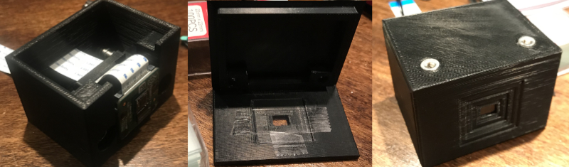
One lensless imaging setup is the DiffuserCam, which has a nice accessible tutorial on building one cheaply. Instead of a lens, this camera design relies on some double-sided scotch tape to diffuse light onto a Raspberry Pi camera sensor. I wanted more control of how far my diffuse material was from the sensor than the method described in the tutorial, so I designed and 3D printed a sensor carriage that allows me to adjust this distance.

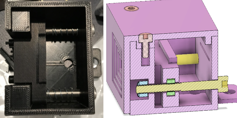
The bolts shown in yellow moves the sensor carriage back and forth. Springs on these same bolts keep the carriage from racking back and forth. The Raspberry Pi camera's lens is removed and attached to the front of the carriage. The double sided tape is attached to a front plate and lid.

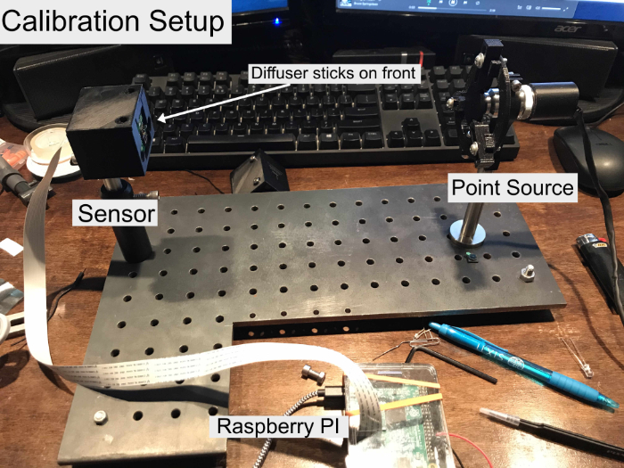
Recovering an image of the scene given the DiffuserCam sensor measurements amounts to a deconvolution problem. While lenses have point spread functions (PSFs) with minimal blurring, a piece of two-sided of scotch tape is far from ideal. I characterized the PSF of my DiffuserCam by constructing a point source out of a white LED, a microscope objective, and a pinhole filter. The Raspberry Pi controlled the brightness of the LED such that the image was bright, but none of the pixels were saturated which would cause distortions. This is the setup and the resulting PSF.

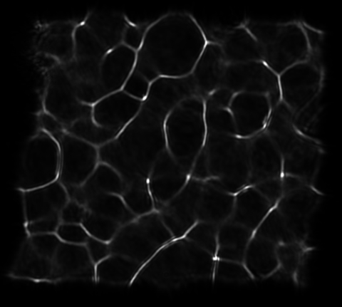
The diffuser blurs a nice point source into a caustic pattern, like one might see at the bottom of a swimming pool on a sunny day. This pattern effectively gets convolved against our scene, and our goal will be to remove it. If we let $\mathbf{x}$ denote our scene, $\mathbf{y}$ our raw sensor measurements, and $\mathbf{b}$ our camera PSF, we can model the image formation as $\mathbf{y} = \mathbf{b} * \mathbf{x} + \mathrm{noise} .$ This problem is underdetermined and ill-conditioned, so we will apply a simple regularizer on our scene (anisotropic $\ell_1$ total variation) and iterative reconstruct the scene $\hat{\mathbf{x}} = \mathrm{arg}\!\min_{\mathbf{x}} \|\mathbf{y} - \mathbf{b} * \mathbf{x} \|_2^2 + \|\mathbf{T}\mathbf{x}\|_{1} .$ Following the work given in the tutorial, we solve this problem using ADMM. To test my camera build, I displayed a University of Michigan block M on my phone screen and took a picture. These are some of my results.

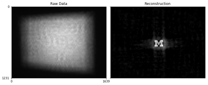
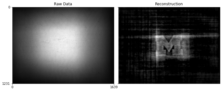
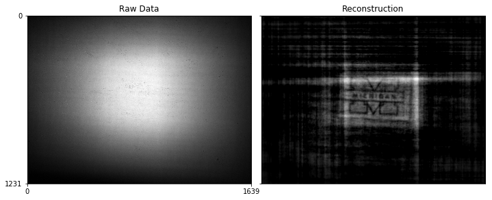
There are a lot of artifacts, especially as the object gets closer, but the Michigan M is clearly identifiable. I could use better regularizers and better optimization algorithms to clean up this more, but I am pretty happy what I have so far. In the future, I may revisit this and get it working on more realistic scenes, but I think its a cool example of non-traditional cameras and computational imaging!